Wie wendet man bedingte Formatierung auf Daten an, die kleiner oder größer als das heutige Datum sind, in Excel?
Die Verwaltung und Nachverfolgung zeitkritischer Informationen ist bei vielen Excel-Aufgaben entscheidend – von der Projektplanung über die Rechnungsstellung mit Fälligkeitsdatum bis hin zur Überwachung von Fristen. Häufig gilt es, Daten, die vor oder nach dem heutigen Datum liegen, visuell klar voneinander zu unterscheiden. Mit der bedingten Formatierung in Excel können Sie solche Daten automatisch hervorheben, sodass überfällige Aufgaben oder anstehende Ereignisse sofort ins Auge fallen – ohne manuelles Scrollen durch Ihre Tabellen. In diesem Tutorial zeigen wir Ihnen mehrere praktische Methoden, um Daten vor oder nach „heute“ effizient hervorzuheben – sowohl mit integrierten Excel-Tools als auch mit erweiterten Lösungen mithilfe von Kutools für Excel. So lernen Sie, Fälligkeitsdaten optimal zu kennzeichnen, zukünftige Aktivitäten klar zu markieren und stets den vollständigen Überblick über Ihre Tabellen zu behalten – unabhängig von Datenvolumen oder Aktualisierungsanforderungen.
- Markieren Sie Daten vor heute oder zukünftige Daten mit Bedingte Formatierung verwenden
- Markieren Sie Daten vor heute oder zukünftige Daten mit KUTOOLS AI
- Kennzeichnen und analysieren Sie Daten mithilfe von Excel-Hilfsspaltenformeln
Markieren Sie Daten vor heute oder zukünftige Daten mit Bedingte Formatierung verwenden
Angenommen, Sie haben eine Spalte mit mehreren Datumsangaben, wie in der folgenden Abbildung dargestellt. Möchten Sie bereits fällige Daten (vor heute) oder zukünftige Termine zur besseren Nachverfolgung und Planung hervorheben, nutzen Sie die bedingte Formatierung in Excel mit Formeln auf Basis der HEUTE-Funktion. Diese Funktion ist besonders wertvoll bei dynamischen Daten, da sich die Formatierung täglich automatisch aktualisiert.

Wählen Sie zunächst Ihre Datenliste aus – in diesem Beispiel die Zellen A2:A15. Klicken Sie auf der Registerkarte Start auf Bedingte Formatierung verwenden > Regeln verwalten. Orientieren Sie sich an der folgenden Abbildung:

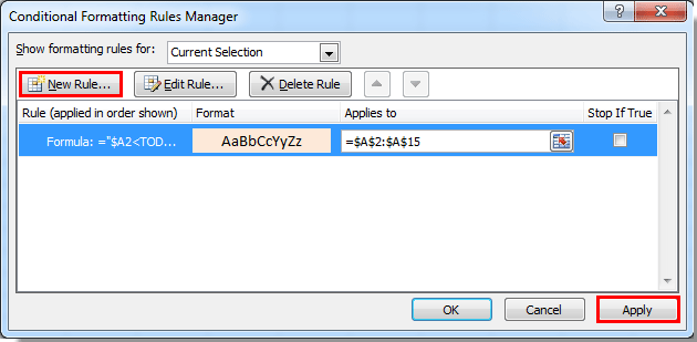
Sobald das Dialogfeld Bedingte Formatierung – Regeln verwalten angezeigt wird, klicken Sie auf die Schaltfläche Neue Regel, um eine benutzerdefinierte, regelbasierte Formel zu erstellen.

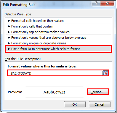
Im Dialogfeld Neue Formatierungsregel:
• Wählen Sie Formel verwenden, um zu bestimmen, welche Zellen formatiert werden sollen. Diese Option ermöglicht eine flexible, datengesteuerte Hervorhebung.
• Um Daten hervorzuheben, die älter als heute sind, kopieren und fügen Sie die folgende Formel in das Feld Formatwerte, bei denen diese Formel zutrifftein:
=$A2<TODAY()• Verwenden Sie zur Hervorhebung von Daten, die nach heute liegen (d. h. anstehende zukünftige Termine), folgende Formel:
=$A2>TODAY()• Klicken Sie anschließend auf die Schaltfläche Format, um Ihr bevorzugtes Erscheinungsbild festzulegen – beispielsweise durch Änderung der Füllfarbe oder des Schriftschnitts. Siehe Beispiel:
Legen Sie Ihre gewünschte Formatierung im Dialogfeld Zellenformat festlegen fest (z. B. wählen Sie eine Farbe, um Fälligkeitsdaten oder zukünftige Daten hervorzuheben), und klicken Sie dann auf OK.
Zurück im Dialogfeld Bedingte Formatierung – Regeln verwalten sehen Sie Ihre neue Regelliste. Um die Regel zu aktivieren, klicken Sie auf Übernehmen. Wenn Sie sowohl überfällige als auch zukünftige Daten hervorheben möchten, wiederholen Sie die Schritte, um eine zweite Regel mit der anderen Formel hinzuzufügen. Beim nächsten Öffnen von „Regeln verwalten“ erscheinen dann beide Regeln.
Nach der Bestätigung mit OK hebt Ihre Excel-Tabelle nun visuell Daten vor und nach heute hervor und liefert klare Hinweise, um gezielte Maßnahmen oder Aufmerksamkeit zu ermöglichen. Sowohl Kennzeichnungen für überfällige als auch für anstehende Termine aktualisieren sich automatisch mit jedem Tag – so behalten Sie stets die relevantesten Elemente auf einen Blick im Fokus.

Hier ist das Ergebnis: Daten, die früher oder später als heute liegen, werden nun entsprechend Ihrer Formatierungsauswahl hervorgehoben – für eine einfachere Überprüfung und Nachverfolgung.

Tipps und Warnhinweise: Stellen Sie sicher, dass Ihre Datumszellen als Datum (nicht als Text) formatiert sind, damit die Formeln korrekt funktionieren. Sollten unerwartete Ergebnisse auftreten, überprüfen Sie Ihr Datumsformat. Bei sehr großen Datensätzen kann die Verwendung bedingter Formatierung die Leistung beeinträchtigen – daher empfiehlt es sich, den Formatierungsbereich möglichst zu begrenzen.
Markieren Sie Daten vor heute oder zukünftige Daten mit KUTOOLS AI
Für Anwender, die eine einfachere und intelligentere Möglichkeit suchen, überfällige oder zukünftige Daten hervorzuheben, vereinfacht KUTOOLS AI für Excel diesen Prozess. Statt manuell Regeln für die bedingte Formatierung zu erstellen, geben Sie KUTOOLS AI Ihre Anweisungen einfach in Klartext ein. Diese Methode ist ideal, wenn Sie regelmäßig Daten hervorheben müssen, dabei Zeit sparen möchten, die manuelle Formeleinrichtung umgehen wollen oder wenn Genauigkeit und Effizienz in Ihrer Arbeitsumgebung oberste Priorität haben.
So verwenden Sie KUTOOLS AI zur Hervorhebung von Daten basierend auf deren Beziehung zum heutigen Tag:
- Klicken Sie auf „Kutools“ > „AI-Assistent“, um den Bereich „KUTOOLS AI Aide“ zu öffnen, und führen Sie dann die folgenden Schritte aus:
- Wählen Sie den Datumsbereich aus, den Sie prüfen möchten.
- Geben Sie im Bereich AI-Assistent einen Befehl wie den folgenden ein:
— Für überfällige Daten:Markieren Sie die Daten vor heute mit hellblauer Farbe in der Bereich auswählen
— Für zukünftige Daten:Markieren Sie die Daten nach heute mit hellblauer Farbe in der Bereich auswählen - Drücken Sie die Eingabetaste oder klicken Sie auf Senden. KUTOOLS AI analysiert Ihre Anfrage. Sobald die Verarbeitung abgeschlossen ist, klicken Sie auf Ausführen, um die Formatierung automatisch anzuwenden.
KUTOOLS AI interpretiert Ihre Absicht automatisch, wählt die geeigneten Formeln und Formate aus und spart Ihnen so Zeit sowie mögliche Fehler bei der manuellen Einrichtung. Dieser Ansatz ist besonders nützlich in dynamischen Arbeitsmappen, für Anwender, die weniger vertraut mit Formeln sind, oder für Personen, die große, häufig aktualisierte Datumslisten verwalten.
Warnhinweis: KUTOOLS AI erfordert eine Internetverbindung und eine aktuelle Installation von Kutools für Excel.
Kennzeichnen und analysieren Sie Daten mithilfe von Excel-Hilfsspaltenformeln
In vielen realen Anwendungsfällen reicht eine einfache farbliche Kennzeichnung oft nicht aus – etwa wenn Sie Datensätze danach filtern, sortieren oder zählen möchten, ob die Daten vor oder nach dem heutigen Datum liegen. Mit Hilfsspalten, die Excel-Formeln enthalten, können Sie solche Fälle klar kennzeichnen und so leistungsstarke Excel-Funktionen wie Filter oder PivotTables für tiefgehende Analysen optimal nutzen.
Vorteile: Einfach einzurichten, unterstützt Sortieren und Filtern und funktioniert in allen Excel-Versionen ohne besondere Berechtigungen.Nachteile: Erfordert zusätzlichen Platz für Hilfsspalten; bietet keine direkte Farbkennzeichnung, es sei denn, sie wird mit bedingter Formatierung kombiniert.
So verwenden Sie eine Hilfsspalte zur schnellen Datumsanalyse:
1. Fügen Sie eine neue Spalte direkt neben Ihrer Datumsliste ein (z. B. Spalte B neben Ihren Daten in A2:A15).
2.Geben Sie in Zelle B2 (angenommen, A2 enthält Ihr erstes Datum) diese Formel ein, um überfällige Daten zu kennzeichnen:
=A2<TODAY()Diese Formel gibt WAHR zurück, wenn das Datum in A2 vor heute liegt, andernfalls FALSCH.
3.Alternativ können Sie zur Kennzeichnung zukünftiger Daten folgende Formel verwenden:
=A2>TODAY()4. Drücken Sie die Eingabetaste, um die Formel zu bestätigen, und ziehen Sie anschließend am Ausfüllkästchen nach unten, um die Spalte für alle Zeilen mit Daten auszufüllen. Mithilfe der WAHR/FALSCH-Ergebnisse können Sie Ihre Datensätze nun ganz einfach nach überfälligen oder anstehenden Aufgaben sortieren oder filtern.
Wenn Sie aussagekräftigere Textkennzeichnungen bevorzugen, ersetzen Sie WAHR/FALSCH durch beschreibendere Markierungen. Beispiel:
=IF(A2<TODAY(),"Overdue",IF(A2>TODAY(),"Upcoming","Today"))Kopieren Sie diese Formel bei Bedarf in alle relevanten Zeilen. Die Spalte können Sie zum Filtern, Sortieren oder als Kriterium in anderen Excel-Funktionen wie der bedingten Formatierung sowie in PivotTables nutzen. Dieser Ansatz eignet sich besonders gut für Berichte, Dashboards oder die Erstellung druckbarer Dokumente.
Hinweis: Befindet sich Ihre Datumsliste nicht in Spalte A, passen Sie die Zellreferenz in der Formel entsprechend an. Stellen Sie sicher, dass der Datentyp Ihrer Datumszellen auf „Datum“ und nicht auf „Text“ eingestellt ist, um inkonsistente Ergebnisse zu vermeiden.
Verwandte Artikel:
- Wie kann man in Excel Zellen basierend auf dem ersten Buchstaben oder Zeichen mit bedingter Formatierung hervorheben?
- Wie kann man in Excel Zellen mit bedingter Formatierung hervorheben, wenn sie den Fehlerwert #NV enthalten?
- Wie kann man das erste Vorkommen in Excel mit bedingter Formatierung hervorheben?
- Wie kann man negative Prozentwerte in Excel mithilfe bedingter Formatierung rot darstellen?
Schnelle Fehlersuchtipps: Wenn Hervorhebungen oder Formeln nicht wie erwartet funktionieren, überprüfen Sie stets Ihre Datumsformatierung und die Bezugsbereiche Ihrer Formeln. Nutzen Sie die Vorschau-Funktion in der bedingten Formatierung, um zu sehen, welche Datensätze betroffen sind, und achten Sie besonders auf doppelte Regeln, die sich überschneiden oder gegenseitig widersprechen könnten. Bei größeren Tabellen können Hilfsspalten oder VBA-Makros die Wartung vereinfachen und wertvolle Zeit sparen – gerade dann, wenn häufige Aktualisierungen anstehen. Testen Sie verschiedene Methoden, um den für Ihr Szenario optimalen Arbeitsablauf zu finden.
Beste Office-Produktivitätstools
Verbessern Sie Ihre Excel-Kenntnisse mit Kutools für Excel und erleben Sie Effizienz wie nie zuvor.Kutools für Excel bietet über 300 erweiterte Funktionen zur Steigerung der Produktivität und Zeit sparen.Klicken Sie hier, um die Funktion zu erhalten, die Sie am dringendsten benötigen...
Office Tab bringt eine tabbasierte Oberfläche in Office und macht Ihre Arbeit viel einfacher
- Aktivieren Sie tabbasiertes Bearbeiten und Lesen in Word, Excel, PowerPoint, Publisher, Access, Visio und Project.
- Öffnen und erstellen Sie mehrere Dokumente in neuen Registerkarten desselben Fensters – statt jedes in einem separaten Fenster zu öffnen.
- Steigert Ihre Produktivität um 50 % und erspart Ihnen täglich Hunderte von Mausklicks!
Alle Kutools-Add-Ins – ein Installationsprogramm
Kutools for Office-Paket bündelt Add-Ins für Excel, Word, Outlook und PowerPoint sowie Office Tab Pro – ideal für Teams, die mit mehreren Office-Anwendungen arbeiten.
- Alles-in-einem-Paket— Add-Ins für Excel, Word, Outlook & PowerPoint sowie Office Tab Pro
- Ein Installationsprogramm, eine Lizenz— innerhalb weniger Minuten eingerichtet (MSI-fähig)
- Funktioniert besser zusammen— optimierte Produktivität über alle Office-Anwendungen hinweg
- 30-tägige Vollversion zum Testen— keine Registrierung, keine Kreditkarte erforderlich
- Bestes Preis-Leistungs-Verhältnis— sparen Sie im Vergleich zum Kauf einzelner Add-Ins