Wie findet man den ersten oder letzten Freitag eines jeden Monats in Excel?
Normalerweise ist Freitag der letzte Arbeitstag des Monats. Wie ermitteln Sie den ersten oder letzten Freitag eines Monats basierend auf einem vorgegebenen Datum in Excel? In diesem Artikel zeigen wir Ihnen Schritt für Schritt, wie Sie mit zwei Formeln den ersten bzw. letzten Freitag jedes Monats finden.
Finden Sie den ersten Freitag eines Monats
Finden Sie den letzten Freitag eines Monats
Finden Sie den ersten Freitag eines Monats
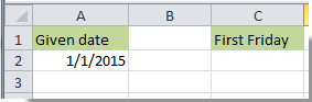
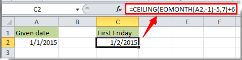
Beispielsweise steht das vorgegebene Datum 01,01.2015 in Zelle A2, wie im folgenden Screenshot gezeigt. Möchten Sie den ersten Freitag des Monats basierend auf diesem Datum ermitteln, gehen Sie wie folgt vor:
1. Wählen Sie eine Zelle aus, um das Ergebnis anzuzeigen – beispielsweise Zelle C2.
2. Kopieren Sie die folgende Formel hinein und drücken Sie Enter.
=CEILING(EOMONTH(A2,-1)-5,7)+6
Hinweise:
Finden Sie den letzten Freitag eines Monats
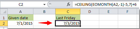
Das vorgegebene Datum 01,01.2015 befindet sich in Zelle A2. So ermitteln Sie in Excel den letzten Freitag dieses Monats:
1. Wählen Sie eine Zelle aus, fügen Sie die folgende Formel ein und drücken Sie die Eingabetaste, um das Ergebnis zu erhalten.
=DATE(YEAR(A2),MONTH(A2)+1,0)+MOD(-WEEKDAY(DATE(YEAR(A2),MONTH(A2)+1,0),2)-2,-7)

Hinweis: Ersetzen Sie A2 in der Formel einfach durch die Bezugszelle Ihres vorgegebenen Datums.
Verwandte Artikel:
- Wie findet man die fünf niedrigsten und höchsten Werte in einer Liste in Excel?
- Wie können Sie prüfen, ob eine bestimmte Arbeitsmappe in Excel geöffnet ist?
- Wie kann man prüfen, ob eine Zelle in Excel von einer anderen Zelle referenziert wird?
- Wie findet man in Excel das Datum in einer Liste, das dem heutigen Datum am nächsten liegt?
Beste Office-Produktivitätstools
Verbessern Sie Ihre Excel-Kenntnisse mit Kutools für Excel und erleben Sie Effizienz wie nie zuvor.Kutools für Excel bietet über 300 erweiterte Funktionen zur Steigerung der Produktivität und Zeit sparen.Klicken Sie hier, um die Funktion zu erhalten, die Sie am dringendsten benötigen...
Office Tab bringt eine tabbasierte Oberfläche in Office und macht Ihre Arbeit viel einfacher
- Aktivieren Sie tabbasiertes Bearbeiten und Lesen in Word, Excel, PowerPoint, Publisher, Access, Visio und Project.
- Öffnen und erstellen Sie mehrere Dokumente in neuen Registerkarten desselben Fensters – statt jedes in einem separaten Fenster zu öffnen.
- Steigert Ihre Produktivität um 50 % und erspart Ihnen täglich Hunderte von Mausklicks!
Alle Kutools-Add-Ins – ein Installationsprogramm
Kutools for Office-Paket bündelt Add-Ins für Excel, Word, Outlook und PowerPoint sowie Office Tab Pro – ideal für Teams, die mit mehreren Office-Anwendungen arbeiten.
- Alles-in-einem-Paket— Add-Ins für Excel, Word, Outlook & PowerPoint sowie Office Tab Pro
- Ein Installationsprogramm, eine Lizenz— innerhalb weniger Minuten eingerichtet (MSI-fähig)
- Funktioniert besser zusammen— optimierte Produktivität über alle Office-Anwendungen hinweg
- 30-tägige Vollversion zum Testen— keine Registrierung, keine Kreditkarte erforderlich
- Bestes Preis-Leistungs-Verhältnis— sparen Sie im Vergleich zum Kauf einzelner Add-Ins