Wie gibt man mit VLOOKUP mehrere Werte in einer einzigen Zelle in Excel zurück?
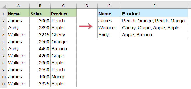
VLOOKUP ist eine leistungsstarke Excel-Funktion, gibt aber standardmäßig nur den ersten übereinstimmenden Wert zurück. Was tun, wenn Sie alle passenden Werte abrufen und in einer einzigen Zelle zusammenführen möchten? Diese Anforderung tritt häufig bei der Analyse von Datensätzen oder beim Zusammenfassen von Informationen auf. In dieser Anleitung zeigen wir Ihnen Schritt für Schritt, wie Sie mithilfe von Formeln und einer praktischen Funktion mehrere Werte in einer einzigen Zelle ausgeben können.
- Alle übereinstimmenden Werte in eine Zelle zusammenführen
- Alle übereinstimmenden Werte ohne Duplikate in eine Zelle zusammenführen
Mehrere Werte mithilfe von Kutools in eine Zelle zusammenführen
Mehrere Werte mit einer benutzerdefinierten Funktion in eine Zelle zusammenführen
- Alle übereinstimmenden Werte in eine Zelle zusammenführen
- Alle übereinstimmenden Werte ohne Duplikate in eine Zelle zusammenführen
Mehrere Werte mit der TEXTVERKETTEN-Funktion in eine Zelle zusammenführen (Excel 2019 und Office 365)
Wenn Sie eine neuere Version von Excel wie Excel 2019 oder Office 365 verwenden, steht Ihnen eine leistungsstarke neue Funktion zur Verfügung: TEXTJOIN. Mit ihr können Sie mithilfe von VLOOKUP im Handumdrehen alle übereinstimmenden Werte in einer einzigen Zelle zusammenführen.
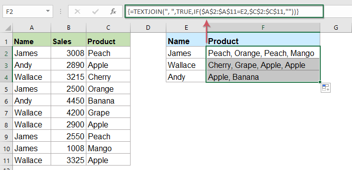
Alle übereinstimmenden Werte in eine Zelle zusammenführen
Wenden Sie die folgende Formel in einer leeren Zelle an, in der das Ergebnis erscheinen soll. Drücken Sie anschließend gleichzeitig STRG + UMSCHALT + EINGABE, um das erste Ergebnis zu erhalten. Ziehen Sie danach den Ausfüllknauf bis zur Zelle, in der Sie die Formel verwenden möchten, und schon erhalten Sie alle zugehörigen Werte – wie im folgenden Screenshot dargestellt:
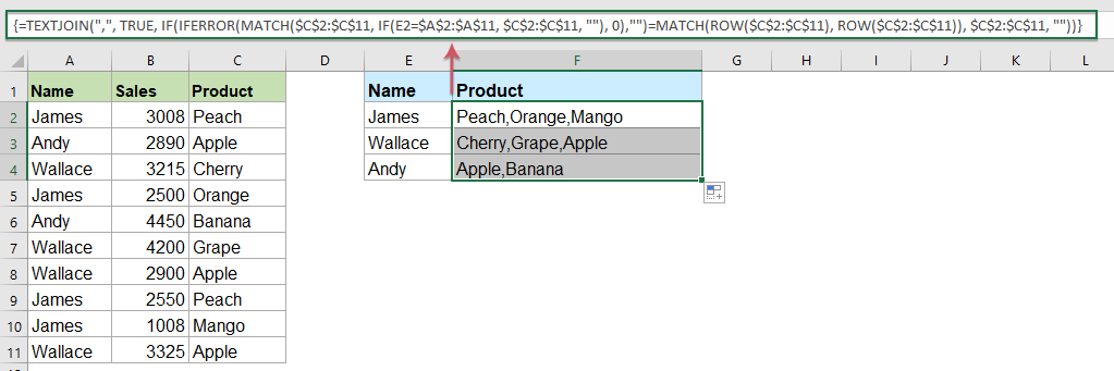
Alle übereinstimmenden Werte ohne Duplikate in eine Zelle zusammenführen
Wenn Sie alle übereinstimmenden Werte basierend auf den Suchkriterien ohne Duplikate erhalten möchten, hilft Ihnen die folgende Formel weiter.
Kopieren Sie die folgende Formel, und fügen Sie sie in eine leere Zelle ein. Drücken Sie anschließend gleichzeitig STRG + UMSCHALT + EINGABE, um das erste Ergebnis zu erhalten. Kopieren Sie diese Formel dann in weitere Zellen – und schon erhalten Sie alle zugehörigen Werte ohne Duplikate, wie im folgenden Screenshot gezeigt:
Mehrere Werte mithilfe von Kutools in eine Zelle zusammenführen
Mit der Funktion „Erweiterte Zeilen zusammenführen“ von Kutools für Excel erhalten Sie mühelos alle übereinstimmenden Werte in einer einzigen Zelle – ganz ohne komplizierte Formeln! Verabschieden Sie sich von zeitaufwändigen manuellen Workarounds und entdecken Sie einen effizienteren Ansatz für Ihre Suchaufgaben in Excel. Lassen Sie uns gemeinsam erkunden, wie Kutools für Excel das möglich macht!
Führen Sie nach der Installation von Kutools für Excel Folgendes aus:
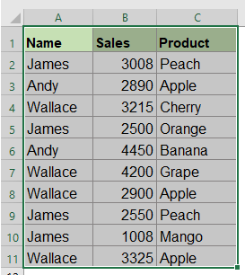
1. Wählen Sie den Datenbereich aus, dessen Spaltenwerte basierend auf einer anderen Spalte zusammengeführt werden sollen.
2. Klicken Sie auf „Kutools“ > „Vereinigen/Aufteilen“ > „Erweiterte Zeilen zusammenführen“ (siehe Screenshot):

3. Führen Sie im erscheinenden Dialogfeld „Erweiterte Zeilen zusammenführen“ die folgenden Schritte aus:
- Klicken Sie auf den Namen der Schlüsselspalte, nach der kombiniert werden soll, und anschließend auf „Primärschlüssel“.
- Klicken Sie anschließend auf eine weitere Spalte, deren Daten basierend auf der Schlüsselspalte kombiniert werden sollen, und wählen Sie im Dropdown-Menü des Feldes „Operation“ im Abschnitt „Kombinieren“ ein Trennzeichen für die zusammengeführten Daten aus.
- Klicken Sie anschließend auf die Schaltfläche „OK“.

Alle zugehörigen Werte aus einer anderen Spalte werden basierend auf dem identischen Wert in einer einzigen Zelle zusammengeführt. Siehe Screenshots:
 |  |
Tipps: Wenn Sie doppelte Inhalte beim Zusammenführen von Zellen entfernen möchten, aktivieren Sie einfach die Option „Doppelte Werte löschen“ im Dialogfeld. So werden nur eindeutige Einträge in einer einzigen Zelle kombiniert – für übersichtlichere und besser organisierte Daten ganz ohne zusätzlichen Aufwand. Siehe Screenshots:
 |  |
Laden Sie Kutools für Excel jetzt herunter und testen Sie es kostenlos!
Mehrere Werte mit einer benutzerdefinierten Funktion in eine Zelle zusammenführen
Die oben genannte TEXTVERKETTEN-Funktion steht nur in Excel 2019 und Office 365 zur Verfügung. Verwenden Sie eine ältere Excel-Version, müssen Sie Code einsetzen, um diese Aufgabe zu erledigen.
Alle übereinstimmenden Werte in eine Zelle zusammenführen
1. Drücken Sie gleichzeitig die Tasten „ALT + F11“, um das Fenster „Microsoft Visual Basic for Applications“ zu öffnen.
2. Klicken Sie auf „Einfügen“ > „Modul“ und fügen Sie den folgenden Code in das Modulfenster ein.
VBA-Code: VLOOKUP, um mehrere Werte in einer Zelle zurückzugeben
Function ConcatenateIf(CriteriaRange As Range, Condition As Variant, ConcatenateRange As Range, Optional Separator As String = ",") As Variant
'Updateby Extendoffice
Dim xResult As String
On Error Resume Next
If CriteriaRange.Count <> ConcatenateRange.Count Then
    ConcatenateIf = CVErr(xlErrRef)
    Exit Function
End If
For i = 1 To CriteriaRange.Count
    If CriteriaRange.Cells(i).Value = Condition Then
        xResult = xResult & Separator & ConcatenateRange.Cells(i).Value
    End If
Next i
If xResult <> "" Then
    xResult = VBA.Mid(xResult, VBA.Len(Separator) + 1)
End If
ConcatenateIf = xResult
Exit Function
End Function
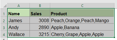
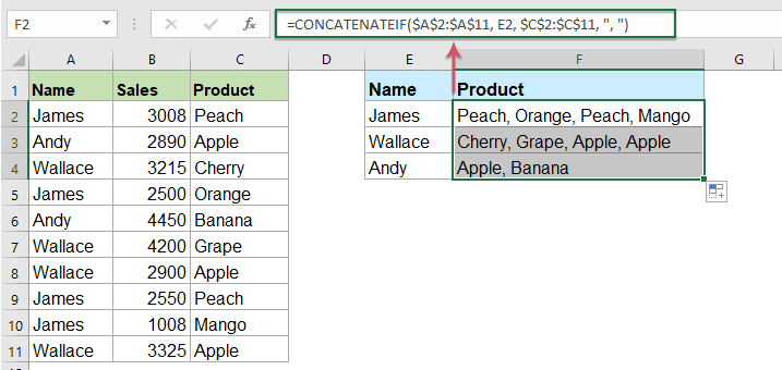
3. Speichern und schließen Sie anschließend diesen Code, kehren Sie zum Arbeitsblatt zurück und geben Sie die folgende Formel in eine leere Zelle Ihrer Wahl ein, um das Ergebnis dort anzuzeigen: =CONCATENATEIF($A$2:$A$11, E2, $C$2:$C$11, ", "). Ziehen Sie dann den Ausfüllknauf nach unten, um alle zugehörigen Werte in jeweils einer Zelle zu erhalten – siehe Screenshot:
Alle übereinstimmenden Werte ohne Duplikate in eine Zelle zusammenführen
Um Duplikate in den zurückgegebenen übereinstimmenden Werten zu ignorieren, verwenden Sie bitte den folgenden Code.
1. Drücken Sie gleichzeitig die Tasten „Alt + F11“, um das Fenster „Microsoft Visual Basic for Applications“ zu öffnen.
2. Klicken Sie auf „Einfügen“ > „Modul“ und fügen Sie den folgenden Code in das Modulfenster ein.
VBA-Code: VLOOKUP und mehrere eindeutige übereinstimmende Werte in einer Zelle zurückgeben
Function MultipleLookupNoRept(Lookupvalue As String, LookupRange As Range, ColumnNumber As Integer)
'Updateby Extendoffice
    Dim xDic As New Dictionary
    Dim xRows As Long
    Dim xStr As String
    Dim i As Long
    On Error Resume Next
    xRows = LookupRange.Rows.Count
    For i = 1 To xRows
        If LookupRange.Columns(1).Cells(i).Value = Lookupvalue Then
            xDic.Add LookupRange.Columns(ColumnNumber).Cells(i).Value, ""
        End If
    Next
    xStr = ""
    MultipleLookupNoRept = xStr
    If xDic.Count > 0 Then
        For i = 0 To xDic.Count - 1
            xStr = xStr & xDic.Keys(i) & ","
        Next
        MultipleLookupNoRept = Left(xStr, Len(xStr) - 1)
    End If
End Function
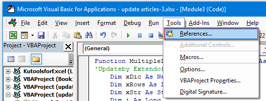
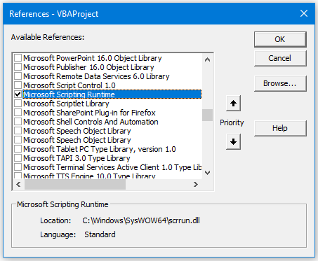
3. Nachdem Sie den Code eingefügt haben, klicken Sie im geöffneten Fenster „Microsoft Visual Basic for Applications“ auf „Extras“ > „Verweise“. Aktivieren Sie im erscheinenden Dialogfeld „Verweise – VBAProject“ die Option „Microsoft Scripting Runtime“ in der Liste „Verfügbare Verweise“ (siehe Screenshots):
 |  |
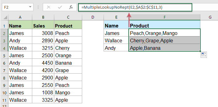
4. Klicken Sie dann auf „OK“, um das Dialogfeld zu schließen, speichern und schließen Sie das Codefenster, kehren Sie zum Arbeitsblatt zurück und geben Sie die folgende Formel in eine leere Zelle ein, in der das Ergebnis angezeigt werden soll: =MultipleLookupNoRept(E2,$A$2:$C$11,3). Ziehen Sie anschließend den Ausfüllknauf nach unten, um alle übereinstimmenden Werte zu erhalten – siehe Screenshot:
Egal, ob Sie Formeln wie TEXTVERKETTEN in Kombination mit Matrixfunktionen verwenden, Tools wie Kutools für Excel einsetzen oder eine benutzerdefinierte Funktion nutzen – alle Ansätze vereinfachen komplexe Suchaufgaben. Wählen Sie die Methode, die am besten zu Ihren Anforderungen passt. Wenn Sie weitere Excel-Tipps und -Tricks entdecken möchten,bietet unsere Website Tausende von Anleitungen.
Weitere verwandte Artikel:
- VLOOKUP-Funktion mit grundlegenden und erweiterten Beispielen
- In Excel ist die VLOOKUP-Funktion eine leistungsstarke Funktion für die meisten Excel-Nutzer. Sie wird verwendet, um in der linken Spalte des Datenbereich nach einem Wert zu suchen und einen passenden Wert aus einer von Ihnen angegebenen Spalte in derselben Zeile zurückzugeben. In diesem Tutorial erfahren Sie, wie Sie die VLOOKUP-Funktion mit einigen grundlegenden und erweiterten Beispielen in Excel verwenden.
- Mehrere übereinstimmende Werte basierend auf einem oder mehreren Kriterien zurückgeben
- Normalerweise ist es für die meisten von uns ein Leichtes, mithilfe der VLOOKUP-Funktion einen bestimmten Wert zu suchen und das zugehörige Element zurückzugeben. Doch haben Sie jemals versucht, mehrere übereinstimmende Werte basierend auf einem oder mehreren Kriterien abzurufen? In diesem Artikel stelle ich Ihnen einige Formeln vor, mit denen Sie diese komplexe Aufgabe in Excel meistern können.
- VLOOKUP und mehrere Werte vertikal zurückgeben
- Normalerweise liefert Ihnen die VLOOKUP-Funktion den ersten passenden Wert. Doch manchmal möchten Sie alle übereinstimmenden Datensätze basierend auf einem bestimmten Kriterium abrufen. In diesem Artikel zeige ich Ihnen, wie Sie mit VLOOKUP alle passenden Werte vertikal, horizontal oder sogar in einer einzigen Zelle ausgeben können.
- VLOOKUP und mehrere Werte aus einer Dropdown-Liste zurückgeben
- Wie können Sie in Excel mithilfe von VLOOKUP mehrere zugehörige Werte aus einer Dropdown-Liste abrufen, sodass beim Auswählen eines Elements alle dazugehörigen Werte sofort angezeigt werden? In diesem Artikel zeige ich Ihnen die Lösung Schritt für Schritt.
Beste Office-Produktivitätstools
Verbessern Sie Ihre Excel-Kenntnisse mit Kutools für Excel und erleben Sie Effizienz wie nie zuvor.Kutools für Excel bietet über 300 erweiterte Funktionen zur Steigerung der Produktivität und Zeit sparen.Klicken Sie hier, um die Funktion zu erhalten, die Sie am dringendsten benötigen...
Office Tab bringt eine tabbasierte Oberfläche in Office und macht Ihre Arbeit viel einfacher
- Aktivieren Sie tabbasiertes Bearbeiten und Lesen in Word, Excel, PowerPoint, Publisher, Access, Visio und Project.
- Öffnen und erstellen Sie mehrere Dokumente in neuen Registerkarten desselben Fensters – statt jedes in einem separaten Fenster zu öffnen.
- Steigert Ihre Produktivität um 50 % und erspart Ihnen täglich Hunderte von Mausklicks!
Alle Kutools-Add-Ins – ein Installationsprogramm
Kutools for Office-Paket bündelt Add-Ins für Excel, Word, Outlook und PowerPoint sowie Office Tab Pro – ideal für Teams, die mit mehreren Office-Anwendungen arbeiten.
- Alles-in-einem-Paket— Add-Ins für Excel, Word, Outlook & PowerPoint sowie Office Tab Pro
- Ein Installationsprogramm, eine Lizenz— innerhalb weniger Minuten eingerichtet (MSI-fähig)
- Funktioniert besser zusammen— optimierte Produktivität über alle Office-Anwendungen hinweg
- 30-tägige Vollversion zum Testen— keine Registrierung, keine Kreditkarte erforderlich
- Bestes Preis-Leistungs-Verhältnis— sparen Sie im Vergleich zum Kauf einzelner Add-Ins