Wie zeigt man in Excel den Namen an, der zur höchsten Punktzahl gehört?
Bei der Analyse von Leistungen oder Ergebnissen in Excel stoßen Sie häufig auf die Notwendigkeit, herauszufinden, welche Person aus einem Datensatz mit Namen und zugehörigen Werten die höchste Punktzahl erreicht hat. Beispielsweise könnten Sie in einer Spalte die Namen der Schüler und in einer anderen deren Testergebnisse haben. Dabei geht es nicht nur darum, die höchste Punktzahl zu ermitteln, sondern auch den Namen (bzw. die Namen im Falle eines Gleichstands) der Person anzuzeigen, die das beste Ergebnis erzielt hat. Dies wird häufig in Szenarien wie der Ermittlung der besten Vertriebsmitarbeiter, bei Schülernoten, Mitarbeiterbewertungen oder in jedem Kontext verwendet, in dem eine Rangfolge wichtig ist.
Im Folgenden stellen wir mehrere praktische Lösungen mit schrittweisen Anleitungen und wertvollen Tipps zur Vermeidung häufiger Fehler vor. Wählen Sie diejenige, die am besten zu Ihrem Datenumfang und Ihren Berichtsanforderungen passt.
Anzeige des zugehörigen Namens der höchsten Punktzahl mithilfe von Formeln
VBA-Code – Automatisches Auffinden und Anzeigen des Namens bzw. der Namen mit der höchsten Punktzahl
Anzeige des zugehörigen Namens der höchsten Punktzahl mithilfe von Formeln
Um den Namen der Person mit der höchsten Punktzahl abzurufen, können Ihnen die folgenden Formeln helfen, das gewünschte Ergebnis zu erhalten. Diese Methode eignet sich für kleine und mittlere Datensätze und funktioniert gut, wenn Sie schnell den besten Leistungsträger identifizieren möchten, ohne zusätzliche Tools einzusetzen.
Verwenden Sie zur Ermittlung des Namens, der der höchsten Punktzahl zugeordnet ist, die Kombination aus INDEXund VERGLEICHwie folgt:
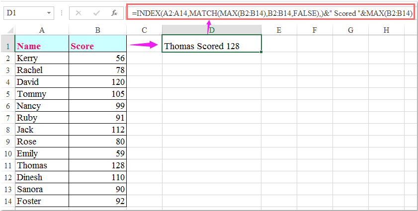
1. Geben Sie die folgende Formel in eine leere Zelle ein, in der der Name angezeigt werden soll (z. B. Zelle C2):
=INDEX(A2:A14,MATCH(MAX(B2:B14),B2:B14,FALSE))&" Scored "&MAX(B2:B14)Nachdem Sie die Formel eingegeben haben, drücken Sie Enter, um die Eingabe zu bestätigen. Die Formel gibt den ersten Vornamen zurück, den sie mit der höchsten Punktzahl findet. Wenn beispielsweise sowohl John als auch Alice 98 Punkte erreicht haben, liefert diese Formel nur den ersten Treffer.
Hinweise:
1. In der obigen Formel ist A2:A14 die Namensliste, aus der Sie den Namen abrufen möchten, und B2:B14 die Liste der Punktzahlen. Stellen Sie sicher, dass die Bereiche exakt mit Ihren Daten übereinstimmen.
2. Die Formel gibt nur den ersten passenden Namen zurück. Wenn mehrere Personen dieselbe höchste Punktzahl erreichen, möchten Sie möglicherweise alle Namen anzeigen lassen – weiter unten finden Sie eine praktische Lösung dafür.
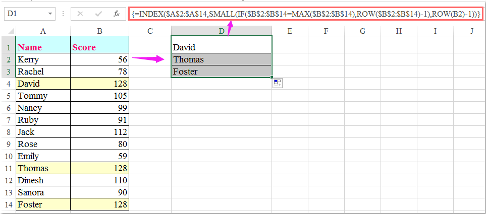
Geben Sie die folgende Formel in eine beliebige Zelle ein (z. B. D2):
=INDEX($A$2:$A$14,SMALL(IF($B$2:$B$14=MAX($B$2:$B$14),ROW($B$2:$B$14)-1),ROW(B2)-1))Nach der Eingabe der Formel drücken Sie gleichzeitig Strg + Umschalt + Enter (nicht nur Enter), um daraus eine Matrixformel zu erstellen. Daraufhin wird der Vorname mit der höchsten Punktzahl angezeigt. Markieren Sie anschließend die Formelzelle und ziehen Sie den Ausfüllknauf nach unten – so lange, bis Fehlerwerte erscheinen. Jede Zeile listet dann eine weitere Person auf, die die höchste Punktzahl erreicht hat. Besonders praktisch ist das bei Gleichständen, wenn Sie alle Gewinner anzeigen möchten.
Wenn Ihre Excel-Version dynamische Arrays unterstützt (z. B. Office 365 oder Excel 2021 und neuer), steht Ihnen ein einfacherer Ansatz zur Verfügung. Geben Sie diese Formel einfach in eine Zelle ein und drücken Sie Enter:
=FILTER(A2:A14,B2:B14=MAX(B2:B14))Diese Formel füllt automatisch alle Namen der Besten in die darunterliegenden Zellen ein – ganz ohne manuelles Ziehen oder spezielle Tastenkombinationen. Praktisch und effektiv für die neuesten Excel-Versionen.
Formeln sind leistungsstark für schnelle Abfragen, eignen sich jedoch möglicherweise nicht optimal für sehr große Datensätze, da die Leistung beeinträchtigt werden kann, wenn Tausende von Zeilen verarbeitet werden. Außerdem erfordern Formeln konsistente Bereichsbezüge, um korrekte Ergebnisse zu liefern, wenn Zeilen hinzugefügt oder entfernt werden – überprüfen Sie daher stets sorgfältig Ihre Datenauswahl.
VBA-Code – Automatisches Auffinden und Anzeigen des Namens bzw. der Namen mit der höchsten Punktzahl
VBA-Makros bieten eine flexible und automatisierte Lösung, um alle Namen zu finden und anzuzeigen, die der höchsten Punktzahl in Ihrem Datensatz entsprechen – besonders dann, wenn Formeln zu komplex oder für umfangreiche Listen ungeeignet sind. Mit VBA passen Sie die Logik ganz einfach Ihren Berichtsanforderungen an und verarbeiten Aktualisierungen automatisch, was sie ideal für wiederkehrende Analysen oder Batch-Verarbeitungen macht.
1. Öffnen Sie Ihre Excel-Arbeitsmappe und klicken Sie anschließend auf Entwicklertools > Visual Basic. Klicken Sie im Fenster Microsoft Visual Basic für Applikationen auf Einfügen > Modul, um ein leeres Modul einzufügen.
Kopieren Sie den folgenden VBA-Code und fügen Sie ihn in das Modulfenster ein:
Sub ShowTopNames()
    Dim rngNames As Range, rngScores As Range, outCell As Range
    Dim nArr As Variant, sArr As Variant
    Dim i As Long, maxVal As Double, hasVal As Boolean
    Dim namesBuf As String
    On Error Resume Next
    Set rngNames = Application.InputBox("Please select the name column (single column)", "Top Names", Type:=8)
    Set rngScores = Application.InputBox("Please select the score column (single column, same rows as names)", "Top Names", Type:=8)
    Set outCell = Application.InputBox("Please select the output cell (optional, click Cancel to skip)", "Top Names", Type:=8)
    On Error GoTo 0
    If rngNames Is Nothing Or rngScores Is Nothing Then Exit Sub
    If rngNames.Rows.Count <> rngScores.Rows.Count Or rngNames.Columns.Count <> 1 Or rngScores.Columns.Count <> 1 Then
        MsgBox "Range mismatch: Name column and score column must be single columns with the same number of rows.", vbExclamation
        Exit Sub
    End If
    nArr = rngNames.Value2
    sArr = rngScores.Value2
    hasVal = False
    For i = 1 To UBound(sArr, 1)
        If IsNumeric(sArr(i, 1)) And Not IsEmpty(sArr(i, 1)) Then
            If Not hasVal Then
                maxVal = CDbl(sArr(i, 1))
                hasVal = True
            ElseIf CDbl(sArr(i, 1)) > maxVal Then
                maxVal = CDbl(sArr(i, 1))
            End If
        End If
    Next i
    If Not hasVal Then
        MsgBox "No valid numeric values found in the score column.", vbInformation
        Exit Sub
    End If
    rngNames.EntireRow.Interior.ColorIndex = xlNone
    For i = 1 To UBound(sArr, 1)
        If IsNumeric(sArr(i, 1)) Then
            If CDbl(sArr(i, 1)) = maxVal Then
                rngNames.Cells(i, 1).EntireRow.Interior.Color = RGB(255, 255, 153) ' Light yellow
                If Len(namesBuf) > 0 Then namesBuf = namesBuf & ", "
                namesBuf = namesBuf & CStr(nArr(i, 1))
            End If
        End If
    Next i
    If Not outCell Is Nothing Then
        outCell.Value = "Top Score: " & maxVal & " | Name(s): " & namesBuf
    End If
    MsgBox "Top Score = " & maxVal & vbCrLf & "Name(s): " & namesBuf, vbInformation, "Highest Score"
End Sub
2. Drücken Sie anschließend die F5-Taste, um diesen Code auszuführen. Es erscheinen drei Eingabeaufforderungen: Wählen Sie die Namensspalte (eine einzelne Spalte). Markieren Sie ausschließlich die Namen (z. B. A2:A14) → OK. Wählen Sie die Punktzahlenspalte (eine einzelne Spalte mit denselben Zeilen wie die Namen). Markieren Sie die Punktzahlen (z. B. B2:B14) → OK. Wählen Sie die Ausgabezelle (optional). Klicken Sie auf eine Zielzelle (z. B. D2), um das Ergebnis dort einzufügen.
Nach Ausführung des Codes wird das Ergebnis in der angegebenen Zelle angezeigt, und die gesamte Zeile aller gleichauf liegenden Spitzenreiter wird hellgelb hervorgehoben.
PivotTable – Verwenden Sie eine PivotTable, um den Namen anzuzeigen, der der höchsten Punktzahl entspricht
PivotTables in Excel bieten eine visuelle und interaktive Möglichkeit, Daten zu analysieren und zusammenzufassen. Sie eignen sich besonders gut für größere Datensätze und Gruppenanalysen sowie zum schnellen Identifizieren eindeutiger Maximalwerte – beispielsweise zur Ermittlung des besten Teilnehmers pro Kategorie oder insgesamt in einer Liste. Diese Methode erfordert weder Formeln noch Programmierkenntnisse und ist daher ideal für Benutzer, die präzise, mausbasierte Lösungen und regelmäßige Berichterstattung bevorzugen.
Der grundlegende Arbeitsablauf zur Verwendung einer PivotTable für diese Anforderung lautet wie folgt:
1. Wählen Sie eine beliebige Zelle innerhalb Ihres Datenbereichs aus (beide Spalten – Namen und Punktzahlen – eingeschlossen) und wechseln Sie dann zu Einfügen > PivotTable. Bestätigen Sie im Dialogfeld den Datenbereich und wählen Sie aus, ob die PivotTable auf einem neuen oder einem vorhandenen Arbeitsblatt platziert werden soll.
2. Ziehen Sie im Bereich „PivotTable-Felder“ das Feld Name in den Bereich Zeilen und das Feld Punktzahl in den Bereich Werte. Standardmäßig wird im Werte-Bereich „Summe“ oder „Anzahl“ verwendet. Klicken Sie auf den Dropdown-Pfeil des Feldes Punktzahl im Werte-Bereich, wählen Sie Wertfeld-Einstellungen und anschließend Max als Zusammenfassungsfunktion aus. Klicken Sie abschließend auf OK.
3. Die PivotTable zeigt nun die höchste Punktzahl für jeden Namen an. Um den absoluten Spitzenreiter hervorzuheben, sortieren Sie die Spalte „Max. von Punktzahl“ absteigend – der oberste Name hat dann die höchste (oder eine gleichhohe) Punktzahl. Zur visuellen Hervorhebung können Sie zudem Filter oder bedingte Formatierung verwenden.
Wenn Sie nur die besten Teilnehmer anzeigen möchten, wenden Sie einen Wertfilter an: Klicken Sie auf den Dropdown-Pfeil bei den Zeilenbeschriftungen für Namen, wählen Sie Wertfilter > Ist gleich und geben Sie den Wert der höchsten Punktzahl ein (den Sie ermitteln können, indem Sie die Werte vorübergehend sortieren oder die höchste Zahl in der Spalte „Max. von Punktzahl“ prüfen). So konzentrieren Sie Ihren Bericht ganz auf die Gewinner.
PivotTables sind ideal für explorative Analysen: Sie können Ihre Daten problemlos aktualisieren, erweitern oder filtern – und die PivotTable berechnet die Ergebnisse automatisch neu. Wenn sich Ihr Datensatz jedoch häufig ändert, denken Sie stets daran, mit der rechten Maustaste auf Ihre PivotTable zu klicken und Aktualisieren auszuwählen, sobald neue Daten hinzugefügt wurden.
PivotTables erfordern zwar etwas Ersteinrichtung, bieten dafür aber flexible Berichterstattung und ermöglichen mühelose Vergleiche zwischen Gruppen – etwa nach Abteilung oder Team –, sofern Ihre Daten zusätzliche Kategorien enthalten.
Falls Probleme bei der Zusammenfassung oder Sortierung auftreten, überprüfen Sie, ob Ihre Daten keine leeren Zellen enthalten und ob die Bedingungsnamen einheitlich geschrieben sind. Bei großen Listen ist besondere Aufmerksamkeit auf den Quellbereich erforderlich, damit die PivotTable alle relevanten Daten berücksichtigt.

Entfesseln Sie die Magie von Excel mit KUTOOLS AI
- Intelligente Ausführung: Führen Sie Zelloperationen durch, analysieren Sie Daten und erstellen Sie Diagramme – alles ganz einfach per Sprachbefehl.
- Benutzerdefinierte Formeln: Erstellen Sie maßgeschneiderte Formeln, um Ihre Arbeitsabläufe optimal zu optimieren.
- VBA-Programmierung: Schreiben und implementieren Sie VBA-Code ganz mühelos.
- Formelinterpretation: Verstehen Sie komplexe Formeln spielend leicht.
- Textübersetzung: Überwinden Sie Sprachbarrieren direkt in Ihren Tabellenkalkulationen.
Beste Office-Produktivitätstools
Verbessern Sie Ihre Excel-Kenntnisse mit Kutools für Excel und erleben Sie Effizienz wie nie zuvor.Kutools für Excel bietet über 300 erweiterte Funktionen zur Steigerung der Produktivität und Zeit sparen.Klicken Sie hier, um die Funktion zu erhalten, die Sie am dringendsten benötigen...
Office Tab bringt eine tabbasierte Oberfläche in Office und macht Ihre Arbeit viel einfacher
- Aktivieren Sie tabbasiertes Bearbeiten und Lesen in Word, Excel, PowerPoint, Publisher, Access, Visio und Project.
- Öffnen und erstellen Sie mehrere Dokumente in neuen Registerkarten desselben Fensters – statt jedes in einem separaten Fenster zu öffnen.
- Steigert Ihre Produktivität um 50 % und erspart Ihnen täglich Hunderte von Mausklicks!
Alle Kutools-Add-Ins – ein Installationsprogramm
Kutools for Office-Paket bündelt Add-Ins für Excel, Word, Outlook und PowerPoint sowie Office Tab Pro – ideal für Teams, die mit mehreren Office-Anwendungen arbeiten.
- Alles-in-einem-Paket— Add-Ins für Excel, Word, Outlook & PowerPoint sowie Office Tab Pro
- Ein Installationsprogramm, eine Lizenz— innerhalb weniger Minuten eingerichtet (MSI-fähig)
- Funktioniert besser zusammen— optimierte Produktivität über alle Office-Anwendungen hinweg
- 30-tägige Vollversion zum Testen— keine Registrierung, keine Kreditkarte erforderlich
- Bestes Preis-Leistungs-Verhältnis— sparen Sie im Vergleich zum Kauf einzelner Add-Ins