Wie findet man die n-te nicht leere Zelle in Excel?
Wie finden und geben Sie den Wert der n-ten nicht leeren Zelle aus einer Spalte oder Zeile in Excel zurück? In diesem Artikel stellen wir Ihnen einige nützliche Formeln vor, die Ihnen diese Aufgabe erleichtern.
Finden und Zurückgeben des Werts der n-ten nicht leeren Zelle aus einer Spalte mithilfe einer Formel
Finden und Zurückgeben des Werts der n-ten nicht leeren Zelle aus einer Zeile mithilfe einer Formel
 Finden und Zurückgeben des Werts der n-ten nicht leeren Zelle aus einer Spalte mithilfe einer Formel
Angenommen, ich habe eine Spalte mit Daten wie im folgenden Screenshot dargestellt. Nun möchte ich den Wert der dritten nicht leeren Zelle aus dieser Liste abrufen.
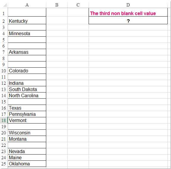
Geben Sie diese Formel in eine leere Zelle ein, in der das Ergebnis ausgegeben werden soll – beispielsweise D2:=INDEX($A$1:$A$25,SMALL(ROW($A$1:$A$25)+(100*($A$1:$A$25="")), 3))&"" Drücken Sie anschließend gleichzeitig die Tasten Strg + Umschalt + Enter, um das korrekte Ergebnis zu erhalten. Siehe Screenshot:

Hinweis: In der obigen Formel ist A1:A25 die Datenliste, die Sie verwenden möchten, und die Zahl 3 gibt an, dass der Wert der dritten nicht leeren Zelle zurückgegeben werden soll. Möchten Sie stattdessen den Wert der zweiten nicht leeren Zelle abrufen, ändern Sie die Zahl einfach von 3 auf 2.
Finden und Zurückgeben des Werts der n-ten nicht leeren Zelle aus einer Zeile mithilfe einer Formel
Wenn Sie den Wert der n-ten nicht leeren Zelle in einer Zeile ermitteln und zurückgeben möchten, unterstützt Sie die folgende Formel dabei. Gehen Sie dazu wie folgt vor:
Geben Sie diese Formel in eine leere Zelle ein, in der das Ergebnis angezeigt werden soll: =INDEX($A$1:$M$1,SMALL(IF($A$1:$M$1<>„",COLUMN($A$1:$M$1)-COLUMN($A$1)+1),4)) Drücken Sie anschließend gleichzeitig die Tasten Strg + Umschalt + Enter, um das Ergebnis zu erhalten. Siehe Screenshot:
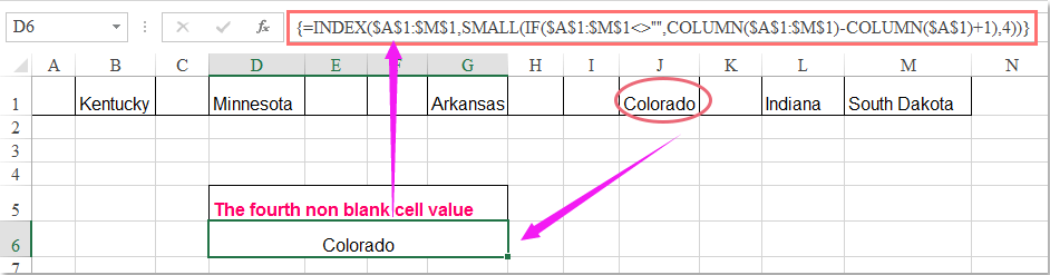
Hinweis: In der obigen Formel ist A1:M1 die Zeile mit den Werten, die Sie verwenden möchten, und die Zahl 4 gibt an, dass der Wert der vierten nicht leeren Zelle zurückgegeben werden soll. Möchten Sie stattdessen den Wert der zweiten nicht leeren Zelle abrufen, ändern Sie die Zahl einfach von 4 auf 2.
Beste Office-Produktivitätstools
Verbessern Sie Ihre Excel-Kenntnisse mit Kutools für Excel und erleben Sie Effizienz wie nie zuvor.Kutools für Excel bietet über 300 erweiterte Funktionen zur Steigerung der Produktivität und Zeit sparen.Klicken Sie hier, um die Funktion zu erhalten, die Sie am dringendsten benötigen...
Office Tab bringt eine tabbasierte Oberfläche in Office und macht Ihre Arbeit viel einfacher
- Aktivieren Sie tabbasiertes Bearbeiten und Lesen in Word, Excel, PowerPoint, Publisher, Access, Visio und Project.
- Öffnen und erstellen Sie mehrere Dokumente in neuen Registerkarten desselben Fensters – statt jedes in einem separaten Fenster zu öffnen.
- Steigert Ihre Produktivität um 50 % und erspart Ihnen täglich Hunderte von Mausklicks!
Alle Kutools-Add-Ins – ein Installationsprogramm
Kutools for Office-Paket bündelt Add-Ins für Excel, Word, Outlook und PowerPoint sowie Office Tab Pro – ideal für Teams, die mit mehreren Office-Anwendungen arbeiten.
- Alles-in-einem-Paket— Add-Ins für Excel, Word, Outlook & PowerPoint sowie Office Tab Pro
- Ein Installationsprogramm, eine Lizenz— innerhalb weniger Minuten eingerichtet (MSI-fähig)
- Funktioniert besser zusammen— optimierte Produktivität über alle Office-Anwendungen hinweg
- 30-tägige Vollversion zum Testen— keine Registrierung, keine Kreditkarte erforderlich
- Bestes Preis-Leistungs-Verhältnis— sparen Sie im Vergleich zum Kauf einzelner Add-Ins