Wie summiert man in Excel anhand von Spalten- und Zeilenkriterien?
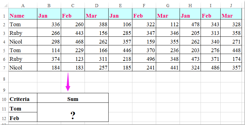
Ich habe einen Datenbereich mit Zeilen- und Spaltenüberschriften und möchte die Summe der Zellen berechnen, die sowohl das Spalten- als auch das Zeilenkriterium erfüllen – beispielsweise alle Zellen, deren Spaltenüberschrift „Tom“ und deren Zeilenüberschrift „Feb“ lautet (siehe folgender Screenshot). In diesem Artikel stelle ich einige nützliche Formeln vor, um dieses Problem zu lösen.
Summieren von Zellen basierend auf Spalten- und Zeilenkriterien mithilfe von Formeln
 Summieren von Zellen basierend auf Spalten- und Zeilenkriterien mithilfe von Formeln
Hier können Sie die folgenden Formeln nutzen, um Zellen anhand beider Kriterien – Spalte und Zeile – zu summieren. Gehen Sie dazu wie folgt vor:
Geben Sie eine der folgenden Formeln in eine leere Zelle ein, in der das Ergebnis ausgegeben werden soll:
=SUMPRODUCT((A2:A7="Tom")*(B1:J1="Feb")*(B2:J7))
=SUM(IF(B1:J1="Feb",IF(A2:A7="Tom",B2:J7)))
Drücken Sie anschließend gleichzeitig die Tasten Umschalttaste + Strg + Enter, um das Ergebnis zu erhalten (siehe Screenshot):
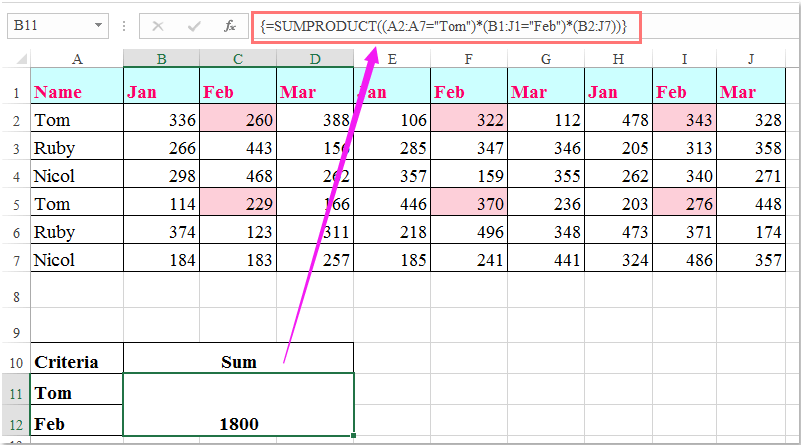
Hinweis: In den obigen Formeln stehen Tom und Feb für das Spalten- bzw. Zeilenkriterium, A2:A7 und B1:J1 sind die Bereiche mit den Spalten- und Zeilenüberschriften, die die Kriterien enthalten, und B2:J7 ist der Datenbereich, den Sie summieren möchten.

Entfesseln Sie die Magie von Excel mit KUTOOLS AI
- Intelligente Ausführung: Führen Sie Zelloperationen durch, analysieren Sie Daten und erstellen Sie Diagramme – alles ganz einfach per Sprachbefehl.
- Benutzerdefinierte Formeln: Erstellen Sie maßgeschneiderte Formeln, um Ihre Arbeitsabläufe optimal zu optimieren.
- VBA-Programmierung: Schreiben und implementieren Sie VBA-Code ganz mühelos.
- Formelinterpretation: Verstehen Sie komplexe Formeln spielend leicht.
- Textübersetzung: Überwinden Sie Sprachbarrieren direkt in Ihren Tabellenkalkulationen.
Beste Office-Produktivitätstools
Verbessern Sie Ihre Excel-Kenntnisse mit Kutools für Excel und erleben Sie Effizienz wie nie zuvor.Kutools für Excel bietet über 300 erweiterte Funktionen zur Steigerung der Produktivität und Zeit sparen.Klicken Sie hier, um die Funktion zu erhalten, die Sie am dringendsten benötigen...
Office Tab bringt eine tabbasierte Oberfläche in Office und macht Ihre Arbeit viel einfacher
- Aktivieren Sie tabbasiertes Bearbeiten und Lesen in Word, Excel, PowerPoint, Publisher, Access, Visio und Project.
- Öffnen und erstellen Sie mehrere Dokumente in neuen Registerkarten desselben Fensters – statt jedes in einem separaten Fenster zu öffnen.
- Steigert Ihre Produktivität um 50 % und erspart Ihnen täglich Hunderte von Mausklicks!
Alle Kutools-Add-Ins – ein Installationsprogramm
Kutools for Office-Paket bündelt Add-Ins für Excel, Word, Outlook und PowerPoint sowie Office Tab Pro – ideal für Teams, die mit mehreren Office-Anwendungen arbeiten.
- Alles-in-einem-Paket— Add-Ins für Excel, Word, Outlook & PowerPoint sowie Office Tab Pro
- Ein Installationsprogramm, eine Lizenz— innerhalb weniger Minuten eingerichtet (MSI-fähig)
- Funktioniert besser zusammen— optimierte Produktivität über alle Office-Anwendungen hinweg
- 30-tägige Vollversion zum Testen— keine Registrierung, keine Kreditkarte erforderlich
- Bestes Preis-Leistungs-Verhältnis— sparen Sie im Vergleich zum Kauf einzelner Add-Ins