Wie geht man vor, wenn eine Zelle ein Wort enthält und anschließend Text in eine andere Zelle eingefügt werden soll?
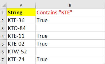
Hier ist eine Liste von Produkt-IDs. Ich möchte prüfen, ob eine Zelle die Zeichenfolge „KTE“ enthält, und anschließend in der benachbarten Zelle „WAHR“ eintragen – wie im folgenden Screenshot gezeigt. Kennen Sie eine schnelle Methode dafür? In diesem Artikel stelle ich Ihnen verschiedene Tricks vor, um zu überprüfen, ob eine Zelle ein bestimmtes Wort enthält, und danach automatisch einen Text in die benachbarte Zelle einzufügen.
Wenn eine Zelle ein Wort enthält, dann entspricht eine andere Zelle einem bestimmten Text
Hier ist eine einfache Formel, mit der Sie schnell prüfen können, ob eine Zelle ein Wort enthält, und danach direkt einen Text in die nächste Zelle einfügen.
Wählen Sie die Zelle aus, in die Sie den Text einfügen möchten, und geben Sie folgende Formel ein:=IF(ISNUMBER(SEARCH("KTE",A2)),"True",„")Ziehen Sie anschließend den AutoAusfüll-Griff nach unten auf die Zellen, auf die Sie diese Formel anwenden möchten. Siehe Screenshot:
 | 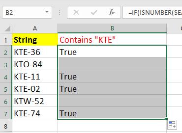 |
In der Formel steht A2 für die Zelle, die Sie auf das Vorkommen eines bestimmten Wortes prüfen möchten; „KTE“ ist das gesuchte Wort, und „WAHR“ der Text, der in einer anderen Zelle angezeigt werden soll. Sie können diese Bezüge jederzeit an Ihre Anforderungen anpassen.
Wenn eine Zelle ein Wort enthält, dann auswählen oder hervorheben
Wenn Sie prüfen möchten, ob eine Zelle ein bestimmtes Wort enthält, und diese anschließend auswählen oder hervorheben wollen, nutzen Sie einfach die Bestimmte Zellen auswählen-Funktion von Kutools für Excel – sie erledigt diese Aufgabe im Handumdrehen.
Nach der Installation von Kutools für Excel führen Sie bitte Folgendes aus:()Kostenlos herunterladen Kutools für Excel jetzt!)
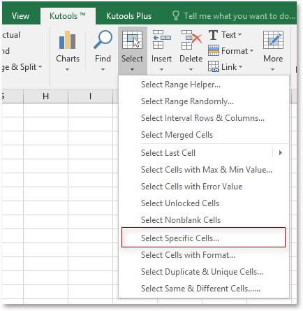
1. Wählen Sie den Bereich aus, in dem Sie prüfen möchten, ob eine Zelle ein bestimmtes Wort enthält, und klicken Sie auf Kutools > Auswählen > Bestimmte Zellen auswählen. Siehe Screenshot:
2. Aktivieren Sie im erscheinenden Dialogfeld die Option Zelle, wählen Sie im ersten Dropdown-Menü enthält aus und geben Sie das gesuchte Wort in das nächste Textfeld ein. Siehe Screenshot: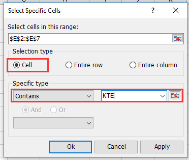
3. Klicken Sie auf OK. Es erscheint ein Dialogfeld, das Ihnen anzeigt, wie viele Zellen das gesuchte Wort enthalten. Klicken Sie auf OK, um das Dialogfeld zu schließen. Siehe Screenshot: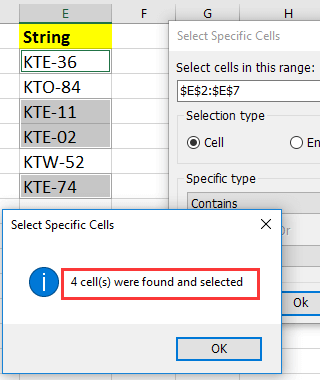
4. Die Zellen, die das angegebene Wort enthalten, sind nun ausgewählt. Wenn Sie sie hervorheben möchten, wechseln Sie zu Start > Füllfarbe, um eine Füllfarbe zur Hervorhebung auszuwählen.
Demo: Bestimmte Zellen auswählen in Excel
Beste Office-Produktivitätstools
Verbessern Sie Ihre Excel-Kenntnisse mit Kutools für Excel und erleben Sie Effizienz wie nie zuvor.Kutools für Excel bietet über 300 erweiterte Funktionen zur Steigerung der Produktivität und Zeit sparen.Klicken Sie hier, um die Funktion zu erhalten, die Sie am dringendsten benötigen...
Office Tab bringt eine tabbasierte Oberfläche in Office und macht Ihre Arbeit viel einfacher
- Aktivieren Sie tabbasiertes Bearbeiten und Lesen in Word, Excel, PowerPoint, Publisher, Access, Visio und Project.
- Öffnen und erstellen Sie mehrere Dokumente in neuen Registerkarten desselben Fensters – statt jedes in einem separaten Fenster zu öffnen.
- Steigert Ihre Produktivität um 50 % und erspart Ihnen täglich Hunderte von Mausklicks!
Alle Kutools-Add-Ins – ein Installationsprogramm
Kutools for Office-Paket bündelt Add-Ins für Excel, Word, Outlook und PowerPoint sowie Office Tab Pro – ideal für Teams, die mit mehreren Office-Anwendungen arbeiten.
- Alles-in-einem-Paket— Add-Ins für Excel, Word, Outlook & PowerPoint sowie Office Tab Pro
- Ein Installationsprogramm, eine Lizenz— innerhalb weniger Minuten eingerichtet (MSI-fähig)
- Funktioniert besser zusammen— optimierte Produktivität über alle Office-Anwendungen hinweg
- 30-tägige Vollversion zum Testen— keine Registrierung, keine Kreditkarte erforderlich
- Bestes Preis-Leistungs-Verhältnis— sparen Sie im Vergleich zum Kauf einzelner Add-Ins