Wie wendet man eine bedingte Formatierung in Google Sheets basierend auf Werten eines anderen Arbeitsblatts an?
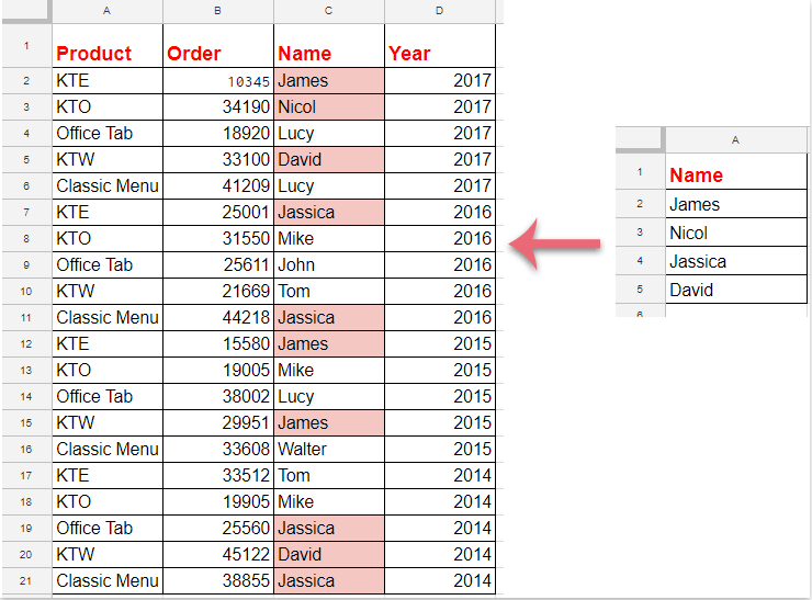
Die bedingte Formatierung ist eine nützliche Funktion in Google Sheets, mit der Sie Zellen automatisch basierend auf bestimmten Kriterien hervorheben können – so lassen sich Ihre Daten leichter analysieren und visualisieren. Manchmal richten sich Ihre Formatierungsregeln jedoch nicht nach Werten innerhalb desselben Arbeitsblatts, sondern nach einer Referenzliste oder Kriterien, die in einem anderen Arbeitsblatt gespeichert sind. Beispielsweise möchten Sie möglicherweise Zellen in einem Arbeitsblatt hervorheben, die auch in einer Liste auftauchen, die in einem anderen Arbeitsblatt verwaltet wird – wie in der folgenden Abbildung dargestellt. Solche Szenarien treten häufig auf, wenn Sie mit verknüpften Daten arbeiten, etwa beim Vergleich aktueller Verkäufe mit einer Master-Produktliste oder beim Prüfen auf doppelte Einträge gegenüber einem anderen Quellbereich. Die Einrichtung einer solchen bedingten Formatierung in Google Sheets – insbesondere bei arbeitsblattübergreifenden Bezügen – kann jedoch verwirrend sein, wenn Sie dies noch nie zuvor gemacht haben. Die folgende Anleitung zeigt Ihnen Schritt für Schritt einen einfachen Ansatz, um genau das zu erreichen.
Bedingte Formatierung verwenden, um Zellen basierend auf einer Liste aus einem anderen Arbeitsblatt in Google Sheets hervorzuheben
Mit dieser Methode können Sie eine Bedingte Formatierung-Regel einrichten, um Zellen in Ihrem Aktuelles Arbeitsblatt hervorzuheben, wenn sie in einer festgelegten Liste eines anderen Arbeitsblatts enthalten sind. Eine solche arbeitsblattübergreifende Bedingte Formatierung verwenden ist besonders nützlich für die dynamische Datenüberwachung und zur Sicherstellung der Konsistenz zwischen verknüpften Datensätzen.
Führen Sie zur Durchführung dieses Vorgangs die folgenden detaillierten Schritte aus:
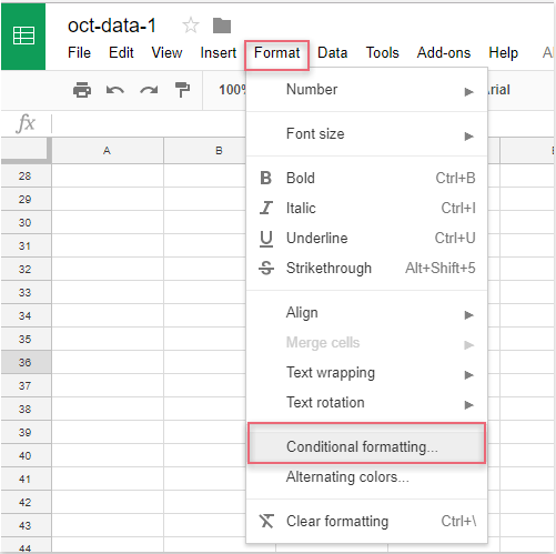
1. Öffnen Sie Ihr Ziellarbeitsblatt und klicken Sie dann im oberen Menü auf Format und wählen Sie Bedingte Formatierung verwenden. Der Bereich Bedingte Formatierung-Regeln öffnet sich auf der rechten Seite Ihres Bildschirms.
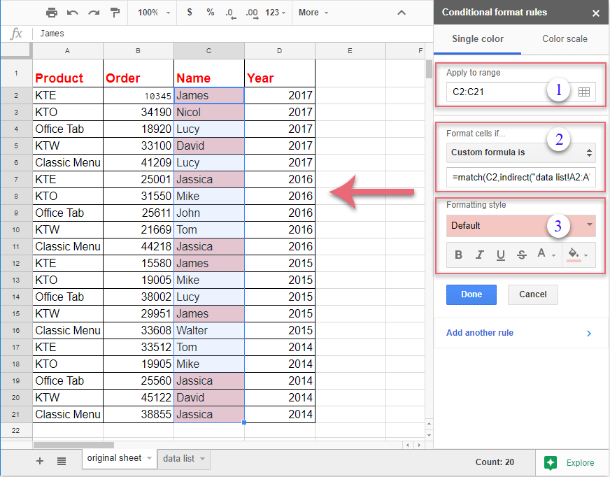
2. Führen Sie im Bereich Bedingte Formatierung – Regeln die folgenden Aktionen aus:
(1.) Klicken Sie auf die Schaltfläche neben dem Feld „Auf Bereich anwenden“, und wählen Sie den Zellbereich aus, den Sie hervorheben möchten. Möchten Sie beispielsweise alle Werte in Spalte C ab Zeile 2 formatieren, wählen Sie  C2:C. Die Auswahl eines geeigneten Bereichs stellt sicher, dass nur die vorgesehenen Zellen für die Formatierung ausgewertet werden.
(2.) Wählen Sie im Dropdown-Menü die Option Zellenformat festlegen, falls Benutzerdefinierte Formel ist. Geben Sie die folgende Formel in das bereitgestellte Feld ein: =MATCH(C2;INDIRECT(„data list!A2:A");0). Diese Formel prüft, ob jede Zelle in Spalte C mit einem beliebigen Wert im Bereich A2:A des Arbeitsblatts „data list“ übereinstimmt.
(3.) Wählen Sie unter Formatierungsstil Ihre gewünschte Formatierung aus, z. B. das Füllen der Zelle mit einer bestimmten Farbe oder das Ändern des Schriftschnitts. Sie können den Stil direkt in Ihrem Arbeitsblatt live anzeigen, bevor Sie ihn anwenden.
Hinweis: In der obigen Formel bezieht sich C2 auf die erste Zelle Ihres ausgewählten Bereichs (passen Sie dies an, falls Ihre Daten in einer anderen Zeile oder Spalte beginnen), und data list!A2:A bezieht sich auf den Arbeitsblattnamen („data list“) und den entsprechenden Bereich (A2:A), in dem Ihre Liste aus dem anderen Arbeitsblatt gespeichert ist. Stellen Sie sicher, dass der Zellbezug in der Formel mit der obersten linken Zelle Ihres ausgewählten Bereichs übereinstimmt, da andernfalls die Formatierung möglicherweise nicht korrekt angewendet wird. Falls sich Ihr Datenlistebereich unterscheidet, aktualisieren Sie ihn bitte in der Formel (z. B. „data list!B2:B“).
3. Sobald Sie die Regel eingerichtet haben, werden übereinstimmende Zellen in Ihrem ausgewählten Bereich sofort basierend auf der Liste des anderen Arbeitsblatts hervorgehoben. Überprüfen Sie die Vorschau und klicken Sie anschließend unten im Bereich FertigBedingte Formatierung-Regeln, um Ihre Formatierung anzuwenden und zu speichern.
Tipps und Fehlerbehebung:
- Überprüfen Sie Ihre Formel sorgfältig auf Tippfehler – insbesondere bei Arbeitsblattnamen und Bereichsbezügen, denn falsche Bezüge sind ein häufiger Grund dafür, dass Regeln nicht angewendet werden.
- Wenn Ihre Datenliste leere Zellen enthält, gibt die
MATCH-Funktion für nicht übereinstimmende Werte einen#N/A-Fehler zurück – das ist jedoch das erwartete Verhalten und beeinträchtigt die Hervorhebung übereinstimmender Elemente nicht. - Wenn Sie zu einem neuen Arbeitsblatt wechseln oder Bereiche anpassen, stellen Sie sicher, dass Sie auch die Zellbezüge in Ihrer benutzerdefinierten Formel entsprechend aktualisieren.
- Die Formatierung aktualisiert sich automatisch, sobald Sie später Elemente aus Ihrer Referenzliste hinzufügen oder entfernen.
- Das in Ihrer Formel referenzierte Arbeitsblatt und der dazugehörige Bereich existieren und sind korrekt geschrieben.
- Die erste Zelle in Ihrer Formel stimmt mit der ersten Zelle Ihres ausgewählten Bereichs überein.
- Alle erforderlichen Berechtigungen für den arbeitsblattübergreifenden Zugriff innerhalb Ihrer Tabellenkalkulation sind vorhanden – diese Methode funktioniert innerhalb einer einzigen, mehrseitigen Google-Sheets-Datei, nicht jedoch über mehrere Dateien hinweg.
Als Alternative können Sie – insbesondere bei komplexeren Datenstrukturen oder Anforderungen wie dem Vergleich mehrerer Spalten, partiellen Übereinstimmungen oder fortgeschrittenen Suchvorgängen – Hilfsspalten mit COUNTIF- oder VLOOKUP-Formeln nutzen oder Google Apps Script (benutzerdefinierten JavaScript-Code) einsetzen, um flexible Lösungen für die bedingte Formatierung zu realisieren.
Zusammenfassend lässt sich sagen, dass die Einrichtung von Bedingte Formatierung verwenden basierend auf einem anderen Arbeitsblatt äußerst effektiv ist für Listenprüfungen, Dublettenverfolgung und diverse arbeitsblattübergreifende Datenvalidierungen – alles innerhalb von Google Sheets. Überprüfen Sie stets Ihre Formeleingaben, Bezugsbereiche und Formatierungsregeln, um reibungslose und genaue Ergebnisse zu erzielen.

Entfesseln Sie die Magie von Excel mit KUTOOLS AI
- Intelligente Ausführung: Führen Sie Zelloperationen durch, analysieren Sie Daten und erstellen Sie Diagramme – alles ganz einfach per Sprachbefehl.
- Benutzerdefinierte Formeln: Erstellen Sie maßgeschneiderte Formeln, um Ihre Arbeitsabläufe optimal zu optimieren.
- VBA-Programmierung: Schreiben und implementieren Sie VBA-Code ganz mühelos.
- Formelinterpretation: Verstehen Sie komplexe Formeln spielend leicht.
- Textübersetzung: Überwinden Sie Sprachbarrieren direkt in Ihren Tabellenkalkulationen.
Beste Office-Produktivitätstools
Verbessern Sie Ihre Excel-Kenntnisse mit Kutools für Excel und erleben Sie Effizienz wie nie zuvor.Kutools für Excel bietet über 300 erweiterte Funktionen zur Steigerung der Produktivität und Zeit sparen.Klicken Sie hier, um die Funktion zu erhalten, die Sie am dringendsten benötigen...
Office Tab bringt eine tabbasierte Oberfläche in Office und macht Ihre Arbeit viel einfacher
- Aktivieren Sie tabbasiertes Bearbeiten und Lesen in Word, Excel, PowerPoint, Publisher, Access, Visio und Project.
- Öffnen und erstellen Sie mehrere Dokumente in neuen Registerkarten desselben Fensters – statt jedes in einem separaten Fenster zu öffnen.
- Steigert Ihre Produktivität um 50 % und erspart Ihnen täglich Hunderte von Mausklicks!
Alle Kutools-Add-Ins – ein Installationsprogramm
Kutools for Office-Paket bündelt Add-Ins für Excel, Word, Outlook und PowerPoint sowie Office Tab Pro – ideal für Teams, die mit mehreren Office-Anwendungen arbeiten.
- Alles-in-einem-Paket— Add-Ins für Excel, Word, Outlook & PowerPoint sowie Office Tab Pro
- Ein Installationsprogramm, eine Lizenz— innerhalb weniger Minuten eingerichtet (MSI-fähig)
- Funktioniert besser zusammen— optimierte Produktivität über alle Office-Anwendungen hinweg
- 30-tägige Vollversion zum Testen— keine Registrierung, keine Kreditkarte erforderlich
- Bestes Preis-Leistungs-Verhältnis— sparen Sie im Vergleich zum Kauf einzelner Add-Ins