Direkt zum Inhalt

Wie kann ich mehrere übereinstimmende Werte basierend auf einem oder mehreren Kriterien in Excel zurückgeben?

Autor: Xiaoyang Letzte Änderung: 2022-07-28

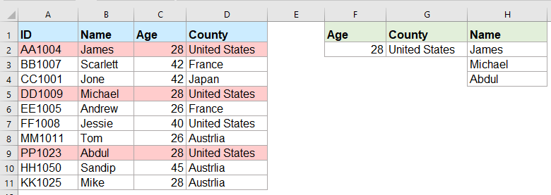
Normalerweise ist es für die meisten von uns einfach, einen bestimmten Wert zu suchen und den passenden Artikel zurückzugeben, indem sie die VLOOKUP-Funktion verwenden. Haben Sie jemals versucht, mehrere übereinstimmende Werte basierend auf einem oder mehreren Kriterien zurückzugeben, wie im folgenden Screenshot gezeigt? In diesem Artikel werde ich einige Formeln zur Lösung dieser komplexen Aufgabe in Excel vorstellen.

Geben Sie mehrere übereinstimmende Werte basierend auf einem oder mehreren Kriterien mit Arrayformeln zurück


Geben Sie mehrere übereinstimmende Werte basierend auf einem oder mehreren Kriterien mit Arrayformeln zurück

Zum Beispiel möchte ich alle Namen extrahieren, die 28 Jahre alt sind und aus den USA stammen. Bitte wenden Sie die folgende Formel an:

1. Kopieren Sie die folgende Formel oder geben Sie sie in eine leere Zelle ein, in der Sie das Ergebnis suchen möchten:

=INDEX($B$2:$B$11, SMALL(IF(COUNTIF($F$2, $C$2:$C$11)*COUNTIF($G$2, $D$2:$D$11), ROW($A$2:$D$11)-MIN(ROW($A$2:$D$11))+1), ROW(A1)), COLUMN(A1))

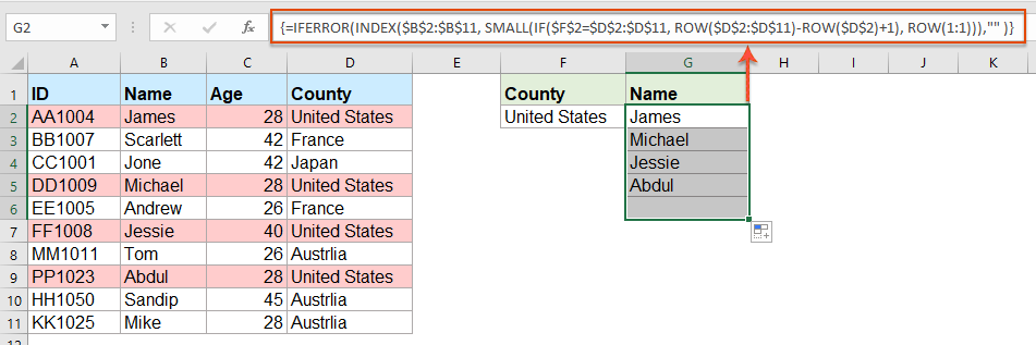
Note: In der obigen Formel B2: B11 ist die Spalte, aus der der übereinstimmende Wert zurückgegeben wird; F2, C2: C11 sind die erste Bedingung und die Spaltendaten, die die erste Bedingung enthalten; G2, D2: D11 Sind die zweite Bedingung und die Spaltendaten, die diese Bedingung enthalten, ändern Sie sie bitte nach Ihren Wünschen.

2. Dann drücken Strg + Umschalt + Enter Geben Sie die Tasten ein, um das erste übereinstimmende Ergebnis zu erhalten. Wählen Sie dann die erste Formelzelle aus und ziehen Sie den Füllpunkt nach unten in die Zellen, bis der Fehlerwert angezeigt wird. Jetzt werden alle übereinstimmenden Werte wie im folgenden Screenshot angezeigt:

Tips: Wenn Sie nur alle übereinstimmenden Werte basierend auf einer Bedingung zurückgeben müssen, wenden Sie bitte die folgende Array-Formel an:

=IFERROR(INDEX($B$2:$B$11, SMALL(IF($F$2=$D$2:$D$11, ROW($D$2:$D$11)-ROW($D$2)+1), ROW(1:1))),"" )


Weitere relative Artikel:

  • Rückgabe mehrerer Suchwerte in einer durch Kommas getrennten Zelle
  • In Excel können wir die VLOOKUP-Funktion anwenden, um den ersten übereinstimmenden Wert aus einer Tabellenzelle zurückzugeben. Manchmal müssen wir jedoch alle übereinstimmenden Werte extrahieren und dann durch ein bestimmtes Trennzeichen wie Komma, Bindestrich usw. in ein einzelnes trennen Zelle wie im folgenden Screenshot gezeigt. Wie können wir in Excel mehrere Suchwerte in einer durch Kommas getrennten Zelle abrufen und zurückgeben?
  • In Google Sheet mehrere übereinstimmende Werte gleichzeitig anzeigen und zurückgeben
  • Die normale Vlookup-Funktion in Google Sheet kann Ihnen helfen, den ersten übereinstimmenden Wert basierend auf bestimmten Daten zu finden und zurückzugeben. Manchmal müssen Sie jedoch alle übereinstimmenden Werte wie im folgenden Screenshot anzeigen und zurückgeben. Haben Sie gute und einfache Möglichkeiten, diese Aufgabe in Google Sheet zu lösen?
  • Anzeigen und Zurückgeben mehrerer Werte aus der Dropdown-Liste
  • Wie können Sie in Excel mehrere entsprechende Werte aus einer Dropdown-Liste anzeigen und zurückgeben? Wenn Sie also ein Element aus der Dropdown-Liste auswählen, werden alle relativen Werte gleichzeitig angezeigt (siehe Abbildung unten). In diesem Artikel werde ich die Lösung Schritt für Schritt vorstellen.
  • Mehrere Werte vertikal in Excel anzeigen und zurückgeben
  • Normalerweise können Sie die Vlookup-Funktion verwenden, um den ersten entsprechenden Wert abzurufen. Manchmal möchten Sie jedoch alle übereinstimmenden Datensätze basierend auf einem bestimmten Kriterium zurückgeben. In diesem Artikel werde ich darüber sprechen, wie alle übereinstimmenden Werte vertikal, horizontal oder in einer einzelnen Zelle angezeigt und zurückgegeben werden.
  • Übereinstimmende Daten zwischen zwei Werten in Excel anzeigen und zurückgeben
  • In Excel können wir die normale Vlookup-Funktion anwenden, um den entsprechenden Wert basierend auf bestimmten Daten zu erhalten. Manchmal möchten wir jedoch den übereinstimmenden Wert zwischen zwei Werten anzeigen und zurückgeben, wie im folgenden Screenshot gezeigt. Wie können Sie mit dieser Aufgabe in Excel umgehen?


  • Super Formelriegel (leicht mehrere Textzeilen und Formeln bearbeiten); Layout lesen (leichtes Lesen und Bearbeiten einer großen Anzahl von Zellen); In gefilterten Bereich einfügen...
  • Zellen / Zeilen / Spalten zusammenführen und Speichern von Daten; Inhalt geteilter Zellen; Kombinieren Sie doppelte Zeilen und Summe / Durchschnitt... doppelte Zellen verhindern; Bereiche vergleichen...
  • Wählen Sie Duplizieren oder Eindeutig Reihen; Wählen Sie Leere Zeilen (alle Zellen sind leer); Super Find und Fuzzy Find in vielen Arbeitsmappen; Zufällige Auswahl ...
  • Exakte Kopie Mehrere Zellen ohne Änderung der Formelreferenz; Referenzen automatisch erstellen zu mehreren Blättern; Aufzählungszeichen einfügen, Kontrollkästchen und mehr ...
  • Lieblingsformeln und schnell einfügen, Bereiche, Diagramme und Bilder; Zellen verschlüsseln mit Passwort; Mailingliste erstellen und E-Mails senden ...
  • Text extrahieren, Text hinzufügen, Nach Position entfernen, Leerzeichen entfernen;; Paging-Zwischensummen erstellen und drucken; Inhalt und Kommentare zwischen Zellen konvertieren...
  • Superfilter (Speichern und Anwenden von Filterschemata auf andere Blätter); Erweiterte Sortierung nach Monat / Woche / Tag, Häufigkeit und mehr; Spezialfilter fett, kursiv ...
  • Kombinieren Sie Arbeitsmappen und Arbeitsblätter;; Tabellen basierend auf Schlüsselspalten zusammenführen; Daten in mehrere Blätter aufteilen; Batch-Konvertierung von xls, xlsx und PDF...
  • Pivot-Tabellengruppierung nach Wochennummer, Wochentag und mehr ... Entsperrte, gesperrte Zellen anzeigen durch verschiedene Farben; Markieren Sie Zellen mit Formel / Name...
kte tab 201905
  • Aktivieren Sie das Bearbeiten und Lesen von Registerkarten in Word, Excel und PowerPoint, Publisher, Access, Visio und Project.
  • Öffnen und erstellen Sie mehrere Dokumente in neuen Registerkarten desselben Fensters und nicht in neuen Fenstern.
  • Steigert Ihre Produktivität um 50 % und reduziert jeden Tag Hunderte von Mausklicks für Sie!
officetab unten


Comments (25)
No ratings yet. Be the first to rate!
This comment was minimized by the moderator on the site
Hi, if there are duplicate values (e.g. two adams), how do i make sure that it only returns 1 adam and not 2?
This comment was minimized by the moderator on the site
Hello, Bobby,
To extract only unique matching values, you should apply the below formula:
After pasting the formula, please press Ctrl + Shift + Enter keys together to get the correct result.
=IFERROR(INDEX($B$2:$B$5, MATCH(0, COUNTIF(H1:$H$1, $B$2:$B$5)+IF($D$2:$D$5<>$G$2, 1, 0)+IF($C$2:$C$5<>$F$2, 1, 0), 0)), "")

Please have a try, hope it can help you!
This comment was minimized by the moderator on the site
Hi,

Thanks for posting these examples.
I'm trying to implement this in my own sheet, but don't get it to work (maybe because I'm using an europe version of excel)?

I want to get the dates of the days that I had my shifts or that I have worked 'some' (>0) hours for a client.

So in I3 is the name and in J3 the month. K3 and L3 are the shifts (1 is worked) and hours (don't know how to set this, should be more than zero)

My expected results are in:
Shifts: I7 and I8
hours: J7

So I worked more than 0 hours for 'person 2' in oktober on 3-10-2022
had shifts for person 2 on '10-10-2022' and 28-10-2022

When I add '=INDEX($B$2:$B$11, SMALL(IF(COUNTIF($F$2, $C$2:$C$11)*COUNTIF($G$2, $D$2:$D$11), ROW($A$2:$D$11)-MIN(ROW($A$2:$D$11))+1), ROW(A1)), COLUMN(A1))' in my excel sheet, it doesn't allow the comma between the different parts of the formula.
So I need to change them to ';'.
But when I try it it always says: '#NAME?'

So can someone help me with this?

Kind regards,

Bas
[img]https://drive.google.com/file/d/1iIPQKuj_PNhqWyWlwJ4IQTqGNEd6B9Hw/view?usp=share_link[/img]
This comment was minimized by the moderator on the site
Hi,

First, thank you for sharing!

Can you please provide a solution to the case below:

I have 3 columns (A: Containing reference information, B: Containing information to be searched, C: Search result)

Image url is provided below

https://ibb.co/VHCd09K

Column A-------------------------Column B------------Column C
File Name-------------------------Name----------------File Name, Document Name, Element Name, Name
Changed Element-----------------Element--------------Changed Element, Element Name, Element ID
Column Location
Document Name
Element Name
Name
Category
Warranty
Slope
Element ID

What I need is to search in column A for any partial match with cell B2 (Name) or B3 (Element) and get the result in one cell,

Thank you, Behzad
This comment was minimized by the moderator on the site
Hello, Behzad
Maybe the below User Defined Function can help you.
Public Function ConcatPartLookUp(rngInput As Range, rngSource As Range, Optional strDelimiter As String, Optional blCaseSensitive)
Dim rng As Range
If strDelimiter = "" Then strDelimiter = ","
If IsMissing(blCaseSensitive) Then
    blCaseSensitive = False
Else
    blCaseSensitive = True
End If
For Each rng In rngSource
    If blCaseSensitive Then
        If InStr(1, rng.Value, rngInput.Value, vbBinaryCompare) > 0 Then ConcatPartLookUp = ConcatPartLookUp & strDelimiter & rng.Value
    Else
        If InStr(1, rng.Value, rngInput.Value, vbTextCompare) > 0 Then ConcatPartLookUp = ConcatPartLookUp & strDelimiter & rng.Value
    End If
Next
If Len(ConcatPartLookUp) > 0 Then ConcatPartLookUp = Mid(ConcatPartLookUp, 2, Len(ConcatPartLookUp))
End Function


After copying and pasting this code, and then use this formula:=ConcatPartLookUp(B2,$A$2:$A$8) to get the result you need.
Please have a try, hope it can help you!
This comment was minimized by the moderator on the site
Heyi, thank you for the formula. It worked for "fixed" values / text as criterias. However, one of the criterias i'm trying to use is a condition (values <>0 ), but does not work the described formula. Do you guys know what should i change to adapt the formula so I can have a condition as one of the criterias, please?

Best,

João
This comment was minimized by the moderator on the site
Hello, Marcus
To solve your problem, please view this article:
https://www.extendoffice.com/documents/excel/6393-excel-vlookup-function.html#b3-2
There are some detailed explanations of this task. You just need to change the criteira to your own.
Thank you!
This comment was minimized by the moderator on the site
Hi,

if in cell H1 i write "Name" and wanted to link that with the formula, how would that work?
Then I could write "ID" in cell H1 and would automatically get as a result: AA1004; DD1009; PP1023 (for the first formula)

Thank you in advance!
This comment was minimized by the moderator on the site
Hello, Marie
Sorry, i can't get the point of your first problem, could you explain your problem more clearly and detailedly? Or you can insert a screenshot here to describe your problem.
As for the second question, you just need to change the cell reference as this:
=INDEX($A$2:$A$11, SMALL(IF(COUNTIF($F$2, $C$2:$C$11)*COUNTIF($G$2, $D$2:$D$11), ROW($A$2:$D$11)-MIN(ROW($A$2:$D$11))+1), ROW(A1)), COLUMN(A1))

Remeber to press Ctrl + Shift + Enter keys together.
Please try, hope it can help you!
This comment was minimized by the moderator on the site
Hello,
what would be needed to expand the first formula in the following case:
Some IDs are Blank (e.g. cell A5 is blank) and I would like an additional condition outputting lines only when the IDs are not blank. (So the output should then be James and Abdul.
Thanks!
This comment was minimized by the moderator on the site
Hello, Jo,
To solve your problem, please apply the below formula:
=INDEX($B$2:$B$11, SMALL(IF(COUNTIF($F$2, $C$2:$C$11)*COUNTIF($G$2, $D$2:$D$11)*($A$2:$A$11<>0), ROW($A$2:$D$11)-MIN(ROW($A$2:$D$11))+1), ROW(A1)), COLUMN(A1))

Please have a ry, hope it can help you!
This comment was minimized by the moderator on the site
hello,
ive tried using the formula and it either generates a value of 0 or the image attached
This comment was minimized by the moderator on the site
Hello, Milku
Your screenshot showed WPS software of MAC version, so I am not sure whether our formula is available.
I uploaded an Excel file to here, you can try to see if it can calculate correctly in you environment.
Thank you!
This comment was minimized by the moderator on the site
When I use the second formula and drag down, nothing appears. The formula result (fx) says it should be returning something but it is blank. How do I correct this?
This comment was minimized by the moderator on the site
Hello Alysia,

Glad to help. I tried the second formula in the article and drag the formula down, the rest of results were returned. I think there may be two reasons for your problem. First, maybe you forget to press Ctrl + Shift + Enter keys to enter the formula. Second, the matching result is only one, so no other results are not returned. Please have a check.

Sincerely,
Mandy
This comment was minimized by the moderator on the site
Hi,

I was wondering if it at all possible to enter a 2nd criteria but from the same range as the 1st criteria,

For example with the used example above i would like to search for the names of people from both America and France So cell F3 would have France, Scarlett & Andrew would also populate in the list in Column G

Thank you for assistance in advance.
This comment was minimized by the moderator on the site
Hello Nick,

Glad to help. If you want to get the names of people from both America and France, I advise you to use our formula twice to get the result. Please see the screenshot, In F2 and G2 are values "United States" and "France". Apply formula =IFERROR(INDEX($B$2:$B$11, SMALL(IF($F$2=$D$2:$D$11, ROW($D$2:$D$11)-ROW($D$2)+1), ROW(1:1))),"" ) to get the results for America. And apply formula =IFERROR(INDEX($B$2:$B$11, SMALL(IF($G$2=$D$2:$D$11, ROW($D$2:$D$11)-ROW($D$2)+1), ROW(1:1))),"" ) to get the results for France. It's simple. Please have a try.

Sincerely,
Mandy
This comment was minimized by the moderator on the site
In the first example, what change to the formula would be needed to return everyone who was less than 28 years old?
There are no comments posted here yet
Load More
Please leave your comments in English
Posting as Guest
×
Rate this post:
0   Characters
Suggested Locations