Wie führt man eine VLOOKUP-Abfrage durch und gibt mehrere zugehörige Werte horizontal in Excel zurück?
VLOOKUP und mehrere Werte horizontal zurückgeben
 VLOOKUP und mehrere Werte horizontal zurückgeben
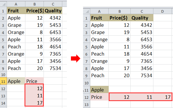
Angenommen, Sie haben einen Datenbereich wie im folgenden Screenshot gezeigt und möchten mithilfe von VLOOKUP die Preise für „Apple“ abrufen.
1. Wählen Sie eine Zelle aus und geben Sie folgende Formel ein:=INDEX($B$2:$B$9; KLEINSTE(WENN($A$11=$A$2:$A$9; ZEILE($A$2:$A$9)-ZEILE($A$2)+1); SPALTE(A1))). Drücken Sie anschließend Umschalt + Strg + Enter und ziehen Sie dann den AutoAusfüll-Griff nach rechts, bis #NUM!erscheint. Siehe Screenshot:
2. Löschen Sie anschließend den Fehlerwert #NUM! (siehe Screenshot).
Tipp: In der obigen Formel ist B2:B9 der Spaltenbereich, aus dem Sie die Werte zurückgeben möchten; A2:A9 der Bereich, in dem sich der Suchwert befindet; A11 der gesuchte Wert; A1 die erste Zelle Ihres Datenbereichs und A2 die erste Zelle des Bereichs, in dem Ihr Suchwert steht.
Wenn Sie mehrere Werte vertikal zurückgeben möchten, können Sie diesen Artikel lesen:Wie sucht man einen Wert und gibt mehrere zugehörige Werte in Excel zurück?

Entfesseln Sie die Magie von Excel mit KUTOOLS AI
- Intelligente Ausführung: Führen Sie Zelloperationen durch, analysieren Sie Daten und erstellen Sie Diagramme – alles ganz einfach per Sprachbefehl.
- Benutzerdefinierte Formeln: Erstellen Sie maßgeschneiderte Formeln, um Ihre Arbeitsabläufe optimal zu optimieren.
- VBA-Programmierung: Schreiben und implementieren Sie VBA-Code ganz mühelos.
- Formelinterpretation: Verstehen Sie komplexe Formeln spielend leicht.
- Textübersetzung: Überwinden Sie Sprachbarrieren direkt in Ihren Tabellenkalkulationen.
Beste Office-Produktivitätstools
Verbessern Sie Ihre Excel-Kenntnisse mit Kutools für Excel und erleben Sie Effizienz wie nie zuvor.Kutools für Excel bietet über 300 erweiterte Funktionen zur Steigerung der Produktivität und Zeit sparen.Klicken Sie hier, um die Funktion zu erhalten, die Sie am dringendsten benötigen...
Office Tab bringt eine tabbasierte Oberfläche in Office und macht Ihre Arbeit viel einfacher
- Aktivieren Sie tabbasiertes Bearbeiten und Lesen in Word, Excel, PowerPoint, Publisher, Access, Visio und Project.
- Öffnen und erstellen Sie mehrere Dokumente in neuen Registerkarten desselben Fensters – statt jedes in einem separaten Fenster zu öffnen.
- Steigert Ihre Produktivität um 50 % und erspart Ihnen täglich Hunderte von Mausklicks!
Alle Kutools-Add-Ins – ein Installationsprogramm
Kutools for Office-Paket bündelt Add-Ins für Excel, Word, Outlook und PowerPoint sowie Office Tab Pro – ideal für Teams, die mit mehreren Office-Anwendungen arbeiten.
- Alles-in-einem-Paket— Add-Ins für Excel, Word, Outlook & PowerPoint sowie Office Tab Pro
- Ein Installationsprogramm, eine Lizenz— innerhalb weniger Minuten eingerichtet (MSI-fähig)
- Funktioniert besser zusammen— optimierte Produktivität über alle Office-Anwendungen hinweg
- 30-tägige Vollversion zum Testen— keine Registrierung, keine Kreditkarte erforderlich
- Bestes Preis-Leistungs-Verhältnis— sparen Sie im Vergleich zum Kauf einzelner Add-Ins